
Notice
Recent Posts
Recent Comments
Link
| 일 | 월 | 화 | 수 | 목 | 금 | 토 |
|---|---|---|---|---|---|---|
| 1 | ||||||
| 2 | 3 | 4 | 5 | 6 | 7 | 8 |
| 9 | 10 | 11 | 12 | 13 | 14 | 15 |
| 16 | 17 | 18 | 19 | 20 | 21 | 22 |
| 23 | 24 | 25 | 26 | 27 | 28 |
Tags
- keda
- MSSQL
- 스프링부트
- blue-green
- logback
- 0 replica
- Strimzi
- eks
- Grafana
- Kafka
- yml
- slow query
- Database
- Benchmarks
- Leaderboard
- spring boot
- SW Maestro
- Debezium
- traceId
- minreplica
- Kubernetes
- zset
- Helm
- 동등성
- docket
- Software maestro
- hammerDB
- propogation
- Salting
- SW 마에스트로
Archives
- Today
- Total
김태오
Linear / Polynomial Regression Model 본문
Importing Packages
from random import random as rand
import random
import numpy as np
import matplotlib.pyplot as plt

%matplotlib inline
Loading Dataset
# Random seed
random.seed(1234)

# Generate 2-dimensional data points
X = [rand() * i * 0.5 - 20 for i in range(0, 100)]
y = [x ** 3 * 0.002 - x ** 2 * 0.005 + x * 0.003 + rand() * 5 for x in X]
print(len(X), len(y))
Random Sampling + Visualization
# Data random shuffle
idx = list(range(len(X)))
random.shuffle(idx)

# Split data for train/test
X_train, X_test = [X[i] for i in idx[:80]], [X[i] for i in idx[80:]]
y_train, y_test = [y[i] for i in idx[:80]], [y[i] for i in idx[80:]]

# 학습 데이터를 시간화해서 분포를 확인해보기
plt.scatter([i for idx, i in enumerate(X_train)],
            [i for idx, i in enumerate(y_train)],
            label='Train', marker='o')

plt.scatter([i for idx, i in enumerate(X_test)],
            [i for idx, i in enumerate(y_test)],
            label='Test', marker='x', color='r')

plt.title('Data points')
plt.xlabel('x')
plt.ylabel('y')
plt.ylim([-20, 20])
plt.legend()
plt.show()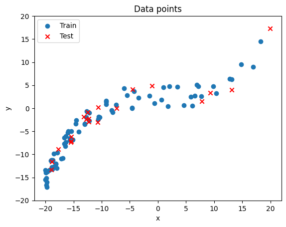
Implementing Linear Regression Model
import math

class Linear():
    def __init__(self):
        self.weight = rand() # Random initialization
        self.bias = 0 # initialization
        self.lr = 5e-4

    def forward(self, x):
        # To compute the weighted sum of Linear regression model
        prediction = self.weight * x  + self.bias
        return prediction

    def backward(self, x, y):
        # To compute the prediction error (derivative of L=1/2 * (prediction - y)^2 by prediction)
        pred = self.forward(x)
        errors = pred - y
        return errors

    def train(self, x, y, epochs):
        for e in range(epochs): # epochs 만큼 학습
            for i in range(len(y)):# Each data point (Online learning)
                x_, y_ = x[i], y[i]

                # To calculate gradient of the model by the sample
                errors = self.backward(x_, y_)
                gradient = errors * x_

                # To update the weight and bias with backward()
                self.weight -= gradient * self.lr
                self.bias -= errors * self.lr

    def evaluate(self, x):
        # To compute the predictions with forward()
        predictions = [self.forward(x_) for x_ in x]
        return predictions # list type
Training + Visualization
# Define a model
linear = Linear()  #  위에서 구현한 Linear regression model 모델 생성

# Training
linear.train(X_train, y_train, 100)   #  100 epoch 학습

# Print weight and bias
print(f"weight: {linear.weight:0.6f}")
print(f"bias: {linear.bias:0.6f}")

# Range of X
x = np.linspace(-20, 20, 50)

# Plotting linear
plt.plot(x, linear.forward(x), label='Prediction')

# Plotting test data points
plt.scatter([i for idx, i in enumerate(X_test)],
            [i for idx, i in enumerate(y_test)],
            label='Test', marker='x', color='r')

# Calculate MSE (Mean Square Error) of test data
mse = sum([(y - linear.forward(x))** 2 for x, y in zip(X_test, y_test)]) / len(X_test)

plt.title(f'Data points (MSE: {mse:0.3f})')
plt.xlabel('x')
plt.ylabel('y')
plt.ylim([-20, 20])
plt.legend()
plt.show()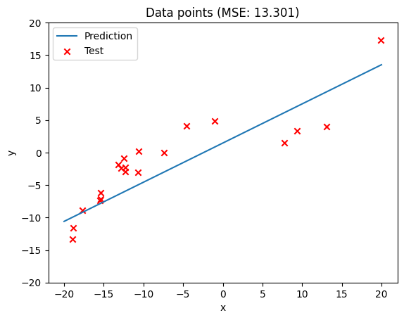
1st Polynomial Regression Model
class Polynomial():
    def __init__(self, dim, lr=1e-5):
        self.dim = dim
        self.weights = [random.random() * 0.001 for i in range(self.dim)] # initialization with a list type
        self.bias = 2.5 # initialization
        self.lr = lr # learning rate

    def forward(self, x):
        # To compute the weighted sum of Polynomial regression model
        prediction = self.bias
        for i in range(self.dim):
            prediction += self.weights[i] * x**(i+1)
        return prediction

    def backward(self, x, y):
        # To compute the prediction error (derivative of L=1/2 * (prediction - y)^2 by prediction)
        pred = self.forward(x)
        errors = pred - y
        return errors

    def train(self, x, y, epochs):
        for e in range(epochs): # epochs 만큼 학습
            for i in range(len(y)): # 데이터 하나씩 학습
                x_, y_ = x[i], y[i] # Each data point

                # To update the weights and bias with backward()
                errors = self.backward(x_, y_)
                for j in range(len(self.weights)):
                    gradient = x_**(j+1) * errors
                    self.weights[j] -=  gradient * self.lr
                self.bias -= errors * self.lr

    def evaluate(self, x):
        # To compute the predictions with forward()
        predictions = [self.forward(x_) for x_ in x]
        return predictions # list type
Implementing Model to get MSE under 3
더보기
dim - Dimensionality of a dataset.
epoch - A complete pass through a training dataset during the training process.
learning rate - The size of the step taken during gradient descent to update the model parameters.
polynomial = Polynomial(dim=2, lr=1e-5)
polynomial.train(X_train, y_train, 200)

# Print weight and bias
for i, weight in enumerate(polynomial.weights):
    print(f"weight_{i+1}: {weight:0.6f}")
print(f"bias: {polynomial.bias:0.6f}")

dim = 3
learning_rate = 1e-9
epochs = range(8000, 16000, 100) # range from 100 to 8000 with an increase of 100

best_mse = float('inf')
best_epoch = None

for epoch in epochs:
    polynomial = Polynomial(dim=dim, lr=learning_rate)
    polynomial.train(X_train, y_train, epoch)
    y_pred = np.array(polynomial.evaluate(X_test))
    mse = np.mean((y_pred - y_test)**2)
    if np.isnan(mse):
        print(f'Skipping epoch={epoch} due to NaN MSE')
        continue
    if mse < best_mse:
        best_mse = mse
        best_epoch = epoch
    print(f'Epoch: {epoch}, MSE: {mse:.3f}')

print(f'Best epoch: {best_epoch}, Best MSE: {best_mse:.3f}')
Best epoch: 8000, Best MSE: 1.838
'ML' 카테고리의 다른 글
| Polynomial Regression (0) | 2023.04.23 |
|---|---|
| Gradient Descent vs. Normal Equation (0) | 2023.04.23 |
| Learning Modes in ML (0) | 2023.04.22 |
| Linear Regression (0) | 2023.04.22 |
| Automatic Differentiation (0) | 2023.04.22 |
'ML' Related Articles
more


